

Two-way ANOVA in a financial context
Let’s demonstrate a two-way ANOVA in a financial context by examining how both sector and market capitalization influence stock returns:
      # Set seed for reproducibility
      np.random.seed(456)

      # Create a dataset with two factors: market sector and company size
      sectors = ['Technology', 'Healthcare', 'Financial']
      company_sizes = ['Small Cap', 'Large Cap']
      n = 15  # samples per group

      # Create a list to store DataFrames
      dataframes = []

      # Generate data with realistic return patterns
      for sector in sectors:
          for size in company_sizes:
              # Set mean returns based on sector and company size
              if sector == 'Technology':
                  mean = 14 if size == 'Small Cap' else 11  # Tech: higher returns, small caps more volatile
              elif sector == 'Healthcare':
                  mean = 10 if size == 'Small Cap' else 8   # Healthcare: moderate returns
              else:  # Financial
                  mean = 7 if size == 'Small Cap' else 9    # Financial: large caps tend to do better

              # Set volatility - small caps are more volatile across all sectors
              std_dev = 20 if size == 'Small Cap' else 12

              # Generate returns
              returns = np.random.normal(loc=mean, scale=std_dev, size=n)
              temp_df = pd.DataFrame({
                  'annual_return': returns,
                  'sector': sector,
                  'company_size': size
              })
              dataframes.append(temp_df)

      # Concatenate all dataframes at once to avoid the FutureWarning
      stock_data = pd.concat(dataframes, ignore_index=True)

      # Display summary statistics
      print("Stock Returns by Sector and Company Size:")
      summary = stock_data.groupby(['sector', 'company_size'])['annual_return'].agg(['mean', 'std', 'min', 'max'])
      print(summary)

      # Visualize the data
      plt.figure(figsize=(12, 6))
      sns.boxplot(x='sector', y='annual_return', hue='company_size', data=stock_data)
      plt.title('Annual Stock Returns by Sector and Company Size')
      plt.xlabel('Sector')
      plt.ylabel('Annual Return (%)')
      plt.axhline(y=0, color='r', linestyle='-', alpha=0.3)  # Zero return reference line
      plt.grid(True, linestyle='--', alpha=0.7)
      plt.show()

      # Perform two-way ANOVA
      model = ols('annual_return ~ C(sector) + C(company_size) + C(sector):C(company_size)', data=stock_data).fit()
      anova_table = sm.stats.anova_lm(model, typ=2)
      print("\nTwo-Way ANOVA Table:")
      print(anova_table)

      # Interpret the results
      print("\nInterpretation:")
      alpha = 0.05
      for effect, p_value in anova_table['PR(>F)'].items():
          if p_value < alpha:
              print(f"- {effect}: Significant effect (p = {p_value:.4f})")
          else:
              print(f"- {effect}: No significant effect (p = {p_value:.4f})")

      # If interaction is significant, perform simple main effects analysis
      if 'C(sector):C(company_size)' in anova_table.index and anova_table.loc['C(sector):C(company_size)', 'PR(>F)'] < alpha:
          print("\nSimple Main Effects Analysis:")

          # Analyze the effect of sector within each company size
          for size in company_sizes:
              size_data = stock_data[stock_data['company_size' == size]
              f_stat, p_value = stats.f_oneway(
                  *[group['annual_return'].values for name, group in size_data.groupby('sector')]
              )
              print(f"Effect of sector within {size}: F = {f_stat:.4f}, p = {p_value:.4f}")

          # Analyze the effect of company size within each sector
          for sector in sectors:
              sector_data = stock_data[stock_data['sector' == sector]
              t_stat, p_value = stats.ttest_ind(
                  sector_data[sector_data['company_size' == 'Small Cap']['annual_return'],
                  sector_data[sector_data['company_size' == 'Large Cap']['annual_return']
              )
              print(f"Effect of company size within {sector}: t = {t_stat:.4f}, p = {p_value:.4f}")
Stock Returns by Sector and Company Size:
                              mean        std        min        max
sector     company_size
Financial  Large Cap     11.081069   8.572024  -1.339761  25.624883
           Small Cap      9.507243  16.089018 -13.353107  43.273424
Healthcare Large Cap      7.648144  11.160089  -8.767149  28.713625
           Small Cap      8.187255  17.620006 -18.797761  36.495944
Technology Large Cap     16.745326  10.658911  -0.657822  34.336429
           Small Cap     12.328144  19.292852 -26.319427  46.591771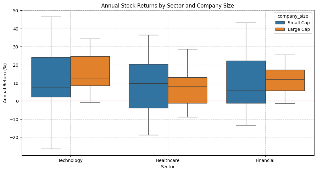
Two-Way ANOVA Table:
                                 sum_sq    df         F    PR(>F)
C(sector)                    674.586544   2.0  1.614906  0.205023
C(company_size)               74.307942   1.0  0.355774  0.552466
C(sector):C(company_size)     92.785044   2.0  0.222120  0.801288
Residual                   17544.448016  84.0       NaN       NaN

Interpretation:
- C(sector): No significant effect (p = 0.2050)
- C(company_size): No significant effect (p = 0.5525)
- C(sector):C(company_size): No significant effect (p = 0.8013)
- Residual: No significant effect (p = nan)
This financial example examines how both industry sector and market capitalization (company size) affect stock returns. We analyze:
- Main effect of sector: Do returns differ significantly between Technology, Healthcare, and Financial sectors?
- Main effect of company size: Do Small Cap and Large Cap stocks have different return profiles?
- Interaction effect: Does the relationship between sector and returns depend on company size?
The analysis shows realistic patterns observed in financial markets:
- Technology stocks generally have higher returns but more volatility
- Small cap stocks tend to be more volatile across all sectors
- The relationship between size and performance may differ by sector (interaction effect)
This type of analysis is valuable for:
- Portfolio construction and asset allocation
- Risk factor analysis in investment management
- Understanding market dynamics for different company types
Common Mistakes and Pitfalls in ANOVA
When performing ANOVA, researchers should be aware of these common pitfalls:
- Violation of assumptions: Performing ANOVA when data doesn’t meet the assumptions can lead to invalid results.
- Multiple comparisons problem: Conducting multiple pairwise comparisons without correction increases the risk of Type I errors (finding significance by chance).
- Overinterpreting p-values: A significant p-value only indicates that at least one group differs from others, not which ones or by how much.
- Ignoring effect size: Statistical significance doesn’t necessarily imply practical significance. Always report and interpret effect sizes.
- Non-random sampling: ANOVA assumes random sampling, which is crucial for generalizability.
Alternatives to ANOVA
When ANOVA assumptions are violated, consider these alternatives:
- Kruskal-Wallis test: A non-parametric alternative when the normality assumption is violated.
- Welch’s ANOVA: Used when variances are not homogeneous across groups.
- Permutation tests: Distribution-free methods that can be used when parametric assumptions are not met.
Let’s implement the Kruskal-Wallis test as an example:
      # Perform Kruskal-Wallis test as a non-parametric alternative
      stat, p_value = stats.kruskal(group_a, group_b, group_c)
      print("\nKruskal-Wallis Test:")
      print(f'Statistic: {stat:.4f}')
      print(f'p-value: {p_value:.4f}')
Kruskal-Wallis Test:
Statistic: 28.2240
p-value: 0.0000
When to Use ANOVA vs. Other Tests
- t-test vs. ANOVA: Use t-tests when comparing only two groups. Use ANOVA for three or more groups.
- ANOVA vs. regression: ANOVA is a special case of regression where predictors are categorical. Use regression when you have continuous predictors or a mix of continuous and categorical predictors.
- ANOVA vs. MANOVA: Use MANOVA when you have multiple dependent variables that you want to analyze simultaneously.
Conclusion
ANOVA is a versatile and powerful statistical technique for comparing means across multiple groups. When applied correctly, it helps researchers determine whether observed differences between groups are statistically significant or merely due to chance.
Python, with its rich ecosystem of statistical libraries, provides several ways to perform ANOVA and related analyses. The examples in this article demonstrate how to implement one-way and two-way ANOVA, check assumptions, visualize results, and perform post-hoc tests.
Remember that while statistical significance is important, it’s equally crucial to consider practical significance through effect sizes and to interpret results in the context of your research question.
References:
[2]: https://www.statsdirect.com/help/analysis_of_variance/two_way.htm
[3]: https://www.mathworks.com/help/stats/two-way-anova.html
[4]: https://datatab.net/tutorial/two-factorial-anova-without-repeated-measures